Previous
1.Tensorflow学习笔记(一) 基础
2.Tensorflow学习笔记(二) Toy Demo
3.Tensorflow学习笔记(三) 使用Skip-Gram和CBOW训练Word Embedding
4.Tensorflow学习笔记(四) 命名实体识别模型(NER-Model)
5.Tensorflow学习笔记(五) RNN语言模型(RNNLM-Model)
Tensorflow学习笔记(六) Tensorboard
由于项目需要,最近又重新开始使用tensorflow了。之前用了一段时间的Keras,觉得很不错,很傻瓜。但是,在具体设计自己的model的时候,还是有很多不方便,因而转到tensorflow来。虽然才过了几个月,但是tensorflow换成1.0之后,很多之前常用的方法都deprecated了,而且有些方法的路径都不太一样,文档也不全。幸亏找了些demo来学,觉得还不错,就记录一下。
Tensorboard demo
代码直接来自:https://github.com/aymericdamien/TensorFlow-Examples/
方便以后直接copy模板,就把代码贴在这里。代码使用的是mnist的例子,会自动下载数据,可能一开始会比较慢一些。windows用户需要修改log路径和数据保存路径。
'''
Graph and Loss visualization using Tensorboard.
This example is using the MNIST database of handwritten digits
(http://yann.lecun.com/exdb/mnist/)
Author: Aymeric Damien
Project: https://github.com/aymericdamien/TensorFlow-Examples/
'''

from __future__ import print_function

import tensorflow as tf

# Import MNIST data
from tensorflow.examples.tutorials.mnist import input_data
mnist = input_data.read_data_sets("/tmp/data/", one_hot=True)

# Parameters
learning_rate = 0.01
training_epochs = 25
batch_size = 100
display_step = 1
logs_path = '/tmp/tensorflow_logs/example'

# Network Parameters
n_hidden_1 = 256 # 1st layer number of features
n_hidden_2 = 256 # 2nd layer number of features
n_input = 784 # MNIST data input (img shape: 28*28)
n_classes = 10 # MNIST total classes (0-9 digits)

# tf Graph Input
# mnist data image of shape 28*28=784
x = tf.placeholder(tf.float32, [None, 784], name='InputData')
# 0-9 digits recognition => 10 classes
y = tf.placeholder(tf.float32, [None, 10], name='LabelData')


# Create model
def multilayer_perceptron(x, weights, biases):
    # Hidden layer with RELU activation
    layer_1 = tf.add(tf.matmul(x, weights['w1']), biases['b1'])
    layer_1 = tf.nn.relu(layer_1)
    # Create a summary to visualize the first layer ReLU activation
    tf.summary.histogram("relu1", layer_1)
    # Hidden layer with RELU activation
    layer_2 = tf.add(tf.matmul(layer_1, weights['w2']), biases['b2'])
    layer_2 = tf.nn.relu(layer_2)
    # Create another summary to visualize the second layer ReLU activation
    tf.summary.histogram("relu2", layer_2)
    # Output layer
    out_layer = tf.add(tf.matmul(layer_2, weights['w3']), biases['b3'])
    return out_layer

# Store layers weight & bias
weights = {
    'w1': tf.Variable(tf.random_normal([n_input, n_hidden_1]), name='W1'),
    'w2': tf.Variable(tf.random_normal([n_hidden_1, n_hidden_2]), name='W2'),
    'w3': tf.Variable(tf.random_normal([n_hidden_2, n_classes]), name='W3')
}
biases = {
    'b1': tf.Variable(tf.random_normal([n_hidden_1]), name='b1'),
    'b2': tf.Variable(tf.random_normal([n_hidden_2]), name='b2'),
    'b3': tf.Variable(tf.random_normal([n_classes]), name='b3')
}

# Encapsulating all ops into scopes, making Tensorboard's Graph
# Visualization more convenient
with tf.name_scope('Model'):
    # Build model
    pred = multilayer_perceptron(x, weights, biases)

with tf.name_scope('Loss'):
    # Softmax Cross entropy (cost function)
    loss = tf.reduce_mean(tf.nn.softmax_cross_entropy_with_logits(labels=y, logits=pred))

with tf.name_scope('SGD'):
    # Gradient Descent
    optimizer = tf.train.GradientDescentOptimizer(learning_rate)
    # Op to calculate every variable gradient
    grads = tf.gradients(loss, tf.trainable_variables())
    grads = list(zip(grads, tf.trainable_variables()))
    # Op to update all variables according to their gradient
    apply_grads = optimizer.apply_gradients(grads_and_vars=grads)

with tf.name_scope('Accuracy'):
    # Accuracy
    acc = tf.equal(tf.argmax(pred, 1), tf.argmax(y, 1))
    acc = tf.reduce_mean(tf.cast(acc, tf.float32))

# Initializing the variables
init = tf.global_variables_initializer()

# Create a summary to monitor cost tensor
tf.summary.scalar("loss", loss)
# Create a summary to monitor accuracy tensor
tf.summary.scalar("accuracy", acc)
# Create summaries to visualize weights
for var in tf.trainable_variables():
    tf.summary.histogram(var.name, var)
# Summarize all gradients
for grad, var in grads:
    tf.summary.histogram(var.name + '/gradient', grad)
# Merge all summaries into a single op
merged_summary_op = tf.summary.merge_all()

# Launch the graph
with tf.Session() as sess:
    sess.run(init)

    # op to write logs to Tensorboard
    summary_writer = tf.summary.FileWriter(logs_path,
                                            graph=tf.get_default_graph())

    # Training cycle
    for epoch in range(training_epochs):
        avg_cost = 0.
        total_batch = int(mnist.train.num_examples/batch_size)
        # Loop over all batches
        for i in range(total_batch):
            batch_xs, batch_ys = mnist.train.next_batch(batch_size)
            # Run optimization op (backprop), cost op (to get loss value)
            # and summary nodes
            _, c, summary = sess.run([apply_grads, loss, merged_summary_op],
                                     feed_dict={x: batch_xs, y: batch_ys})
            # Write logs at every iteration
            summary_writer.add_summary(summary, epoch * total_batch + i)
            # Compute average loss
            avg_cost += c / total_batch
        # Display logs per epoch step
        if (epoch+1) % display_step == 0:
            print("Epoch:", '%04d' % (epoch+1), "cost=", "{:.9f}".format(avg_cost))

    print("Optimization Finished!")

    # Test model
    # Calculate accuracy
    print("Accuracy:", acc.eval({x: mnist.test.images, y: mnist.test.labels}))

    print("Run the command line:\n" \
          "--> tensorboard --logdir=/tmp/tensorflow_logs " \
          "\nThen open http://0.0.0.0:6006/ into your web browser")
结果显示
图和代码稍微有点不匹配(之中改了一下源代码,不然会报错,但是不影响Tensorboard的使用),所以不用在意具体的结果。
1.SCALARS——显示accuracy
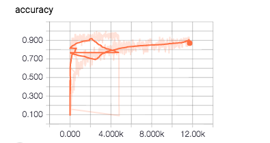
横轴为step(例子中为一个batch一个),纵轴为accuracy
2.SCALARS——显示loss
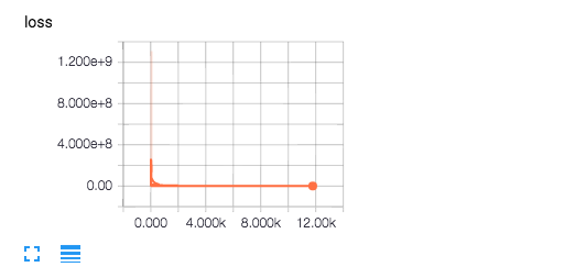
横轴为step,纵轴为loss
3.GRAPHS
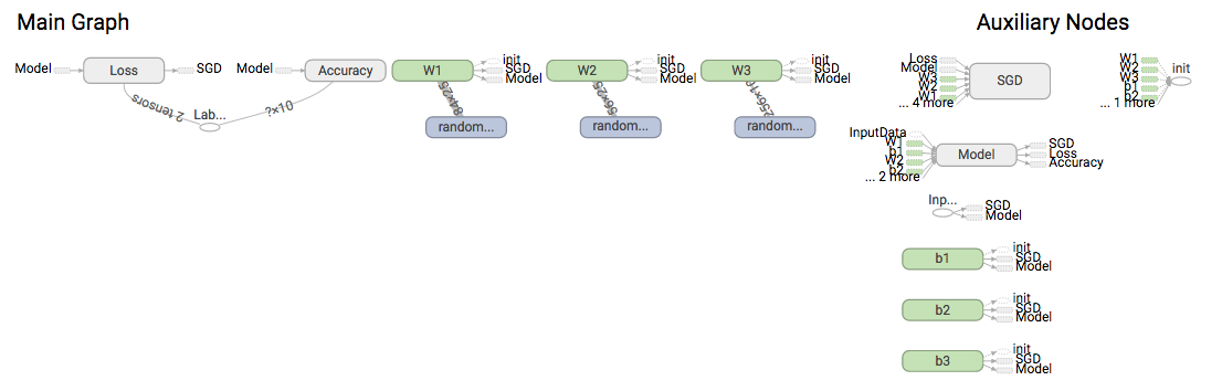
主要用来显示计算图和各个计算节点
4.HISTOGRAMS——可查看weights、biases、gradients、layer outputs
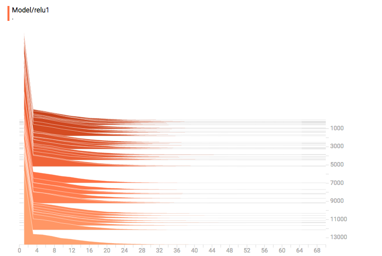
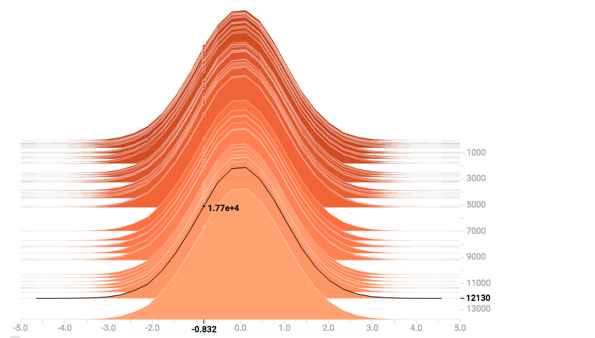
横轴为值,纵轴为step,主要是统计各个step下该参数中的各个值的统计数