ICA算法之算法实现
看了一天的源码+别人写的资料+原始论文(但是还没怎么看……),感觉ICA算法的基本思路比较简单,但是推广到fastICA的时候又遇到各种不明所以的运算步骤,再到算法实现的时候参考sklearn.decomposition下的fastica源码,又有一些不明所以的处理方式。本来觉得一天足够的事情,但是现在看来想要吃透并且深入理解每个细节,还是要花一些功夫的,最好还是看最原始的论文,能更好的理解。
对照了半天的源码和资料,目前算是知道了大部分细节,解释直接放在代码注释里了。ICA的原理我试着整理了一下,另一篇给出简单的推导过程。fastICA目前只是了解大致的算法步骤,具体的数学原理还需要在原论文里考证。原论文为:A. Hyvarinen and E. Oja, Independent Component Analysis: Algorithms and Applications, Neural Networks, 13(4-5), 2000, pp. 411-430。
注意,经过ICA处理后重建的数据,只保证源数据的形状具有相似性,但是幅度可能会不一样,且可能会翻转,或者顺序调换。因为ICA是一个不定问题,有多个解符合假设(特征向量不唯一等因素)。
应用
可以使用该算法对混合的信号进行分离,得到各个独立的信号。比如盲信号分离。
sklearn源码里给出的一段话个人觉得不错:
The data matrix X is considered to be a linear combination of non-Gaussian (independent) components i.e. X = AS where columns of S contain the independent components and A is a linear mixing matrix. In short ICA attempts to `un-mix` the data by estimating an un-mixing matrix W where ``S = W K X.``
注意
能够分离的先决条件是:各个信号独立,非高斯,且接收源的个数(X的大小)等于独立源的个数(S的大小)。
代码
# -*- encoding:utf-8 -*-
import sys
import math
import numpy as np
from matplotlib import pyplot as plt
from sklearn.decomposition import fastica
from copy import deepcopy


class ICA():
    def __init__(self, signalRange, timeRange):
        # 信号幅度
        self.signalRange = signalRange
        # 时间范围
        self.timeRange = timeRange
        # 固定每个单位时间10个点,产生x
        self.x = np.arange(0, self.timeRange, 0.1)
        # 所有的点数
        self.pointNumber = self.x.shape[0]

    # 生成正弦波
    def produceSin(self, period=100, drawable=False):
        y = self.signalRange * np.sin(self.x / period * 2 * np.pi)
        if drawable:
            plt.plot(self.x, y)
            plt.show()

        return y

    # 生成方波
    def produceRect(self, period=20, drawable=False):
        y = np.ones(self.pointNumber) * self.signalRange
        begin = 0
        end = self.pointNumber
        step = period * 10
        mid = step // 2
        while begin < end:
            y[begin:mid] = -1 * self.signalRange
            begin += step
            mid += step
        if drawable:
            plt.plot(self.x, y)
            plt.show()

        return y

    # 生成三角波
    def produceAngle(self, period=20, drawable=False):
        lastPoint = period * 10 - 1
        if lastPoint >= self.pointNumber:
            raise ValueError('You must keep at least one period!')
        delta = ((-1 - 1) * self.signalRange) / float(self.x[lastPoint] - self.x[0])
        y = (self.x[:lastPoint+1] - self.x[0]) * delta + self.signalRange
        y = np.tile(y, self.pointNumber // y.shape[0])[:self.pointNumber]

        if drawable:
            plt.plot(self.x, y)
            plt.show()
        return y

    # 生成uniform噪声
    def produceNoise(self, signalRange=None, drawable=False):
        if signalRange is None:
            signalRange = self.signalRange
        y = np.asarray([(np.random.random() - 0.5) * 2 * signalRange for _ in xrange(self.pointNumber)])

        if drawable:
            plt.plot(self.x, y)
            plt.show()

        return y

    # 混合信号
    def mixSignal(self,majorSignal, *noises, **kwargs):
        mixSig = deepcopy(majorSignal)
        noiseRange = 0.5
        if 'noiseRange' in kwargs and kwargs['noiseRange']:
            noiseRange = kwargs['noiseRange']
        for noise in noises:
            mixSig += noiseRange * np.random.random() * noise
        if 'drawable' in kwargs and kwargs['drawable']:
            plt.plot(self.x, mixSig)
            plt.show()

        return mixSig


    # 让每个信号的样本均值为0,且协方差(各个信号之间)为单位阵
    def whiten(self, X):
        # 加None可以认为是将向量进行转置,但是对于矩阵来说,是在中间插入了一维
        X = X - X.mean(-1)[:, None]
        A = np.dot(X, X.T)
        D, P = np.linalg.eig(A)
        D = np.diag(D)
        D_inv = np.linalg.inv(D)
        D_half = np.sqrt(D_inv)

        V = np.dot(D_half, P.T)

        return np.dot(V, X), V

    # 就是sklearn的源码里面的logcosh
    # 源码里有fun_args,用到一个alpha来调整幅度,这里省略没加
    # tanh(x)的导数为1-tanh(x)^2
    def _tanh(self, x):
        gx = np.tanh(x)
        g_x = gx ** 2
        g_x -= 1
        g_x *= -1
        return gx, g_x.mean(-1)

    def _exp(self, x):
        exp = np.exp(-(x ** 2) / 2)
        gx = x * exp
        g_x = (1 - x ** 2) * exp
        return gx, g_x.mean(axis=-1)


    def _cube(self, x):
        return x ** 3, (3 * x ** 2).mean(axis=-1)

    # W <- (W_1 * W_1')^(-1/2) * W_1
    def decorrelation(self, W):
        U, S = np.linalg.eigh(np.dot(W, W.T))
        U = np.diag(U)
        U_inv = np.linalg.inv(U)
        U_half = np.sqrt(U_inv)
        # rebuild_W = np.dot(np.dot(S * 1. / np.sqrt(U), S.T), W)
        rebuild_W = np.dot(np.dot(np.dot(S, U_half), S.T), W)
        return rebuild_W

    # fastICA
    def fastICA(self, X, fun='tanh'):
        n, m = X.shape
        p = float(m)
        if fun == 'tanh':
            g = self._tanh
        elif fun == 'exp':
            g = self._exp
        elif fun == 'cube':
            g = self._cube
        else:
            raise ValueError('The algorighm does not '
                             'support the support the user-defined function.'
                             'You must choose the function in (`tanh`, `exp`, `cube`)')
        # 不懂, 需要深挖才能知道, sklearn的源码里有这个,查的资料里说是black magic
        X *= np.sqrt(X.shape[1])

        # 随机化W,只要保证非奇异即可,源码里默认使用normal distribution来初始化,对应init_w参数
        W = np.ones((n,n), np.float32)
        for i in range(n):
            for j in range(i):
                W[i,j] = np.random.random()

        # 随机化W的另一种方法,但是这个不保证奇异
        # W = np.random.random((n, n))
        # W = self.decorrelation(W)

        # 迭代计算W
        maxIter = 300
        for ii in range(maxIter):
            gwtx, g_wtx = g(np.dot(W, X))
            W1 = self.decorrelation(np.dot(gwtx, X.T) / p - g_wtx[:, None] * W)
            lim = max(abs(abs(np.diag(np.dot(W1, W.T))) - 1))
            W = W1
            if lim < 0.00001:
                break
        return W

    # 画图
    def draw(self, y, figNum):
        if y.__class__ == list:
            m = len(y)
            n = 0
            if m > 0:
                n = len(y[0])
        elif y.__class__ == np.array([]).__class__:
            m, n = y.shape
        else:
            raise ValueError('The first arg you give must be type of list or np.array.')
        plt.figure(figNum)
        for i in range(m):
            plt.subplot(m, 1, i + 1)
            plt.plot(self.x, y[i])

    # 显示
    def show(self):
        plt.show()


if __name__ == '__main__':
    # 设置信号幅度为2,时间范围为[0, 200)
    ica = ICA(2, 200)
    # 周期为100的正弦波
    gsigSin = ica.produceSin(100, False)
    # 周期为20的方形波
    gsigRect = ica.produceRect(20, False)
    # 周期为20的三角波
    gsigAngle = ica.produceAngle(20, False)
    # 幅度为0.5的uniform噪声
    gsigNoise = ica.produceNoise(0.5, False)
    # 独立信号S
    totalSig = [gsigSin, gsigRect, gsigAngle, gsigNoise]
    # 混合信号X
    mixSig = []
    for i, majorSig in enumerate(totalSig):
        curSig = ica.mixSignal(majorSig, *(totalSig[:i] + totalSig[i+1:]), drawable=False)
        mixSig.append(curSig)
    mixSig = np.asarray(mixSig)


    # 以下是调用自己写的fastICA, 默认做了白化处理,不用白化效果貌似不太行
    xWhiten, V = ica.whiten(mixSig)
    # fun的选择和你假设的S的概率分布函数有关,一般假设为sigmoid函数, 则对应为tanh
    W = ica.fastICA(xWhiten, fun='tanh')
    recoverSig = np.dot(np.dot(W, V), mixSig)
    ica.draw(totalSig, 1)
    ica.draw(mixSig, 2)
    ica.draw(recoverSig, 3)
    ica.show()

    # 以下是调用sklearn包里面的fastICA
    # V对应白化处理的变换矩阵即Z = V * X, W对应S = W * Z
    V, W, S = fastica(mixSig.T)
    # 不做白化处理的话就不用乘K
    assert ((np.dot(np.dot(W, V), mixSig) - S.T) < 0.00001).all()
    ica.draw(totalSig, 1)
    ica.draw(mixSig, 2)
    ica.draw(S.T, 3)
    ica.show()
结果
下面分别观察使用自己写的和使用sklearn包跑出来的不同结果。两者均使用了去均值(相对每个信号自身)和去相关(即白化,是各个信号之间的相关性)。其实可以把每个时间点下各个信号的值看成feature,点的个数就是sample_num。
信号使用了四种:正弦波、方波、三角波和uniform噪声,原始信号如下图:
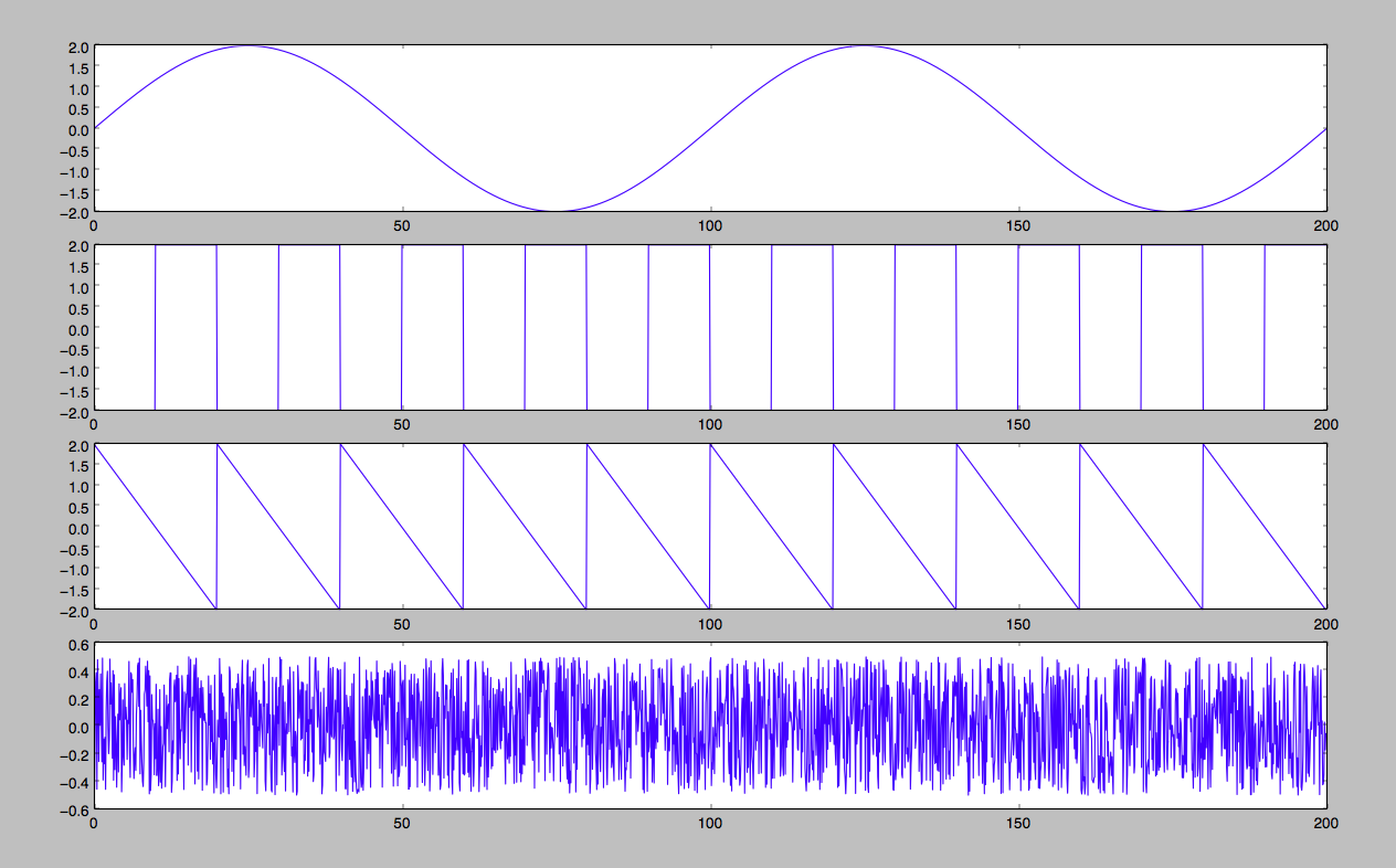
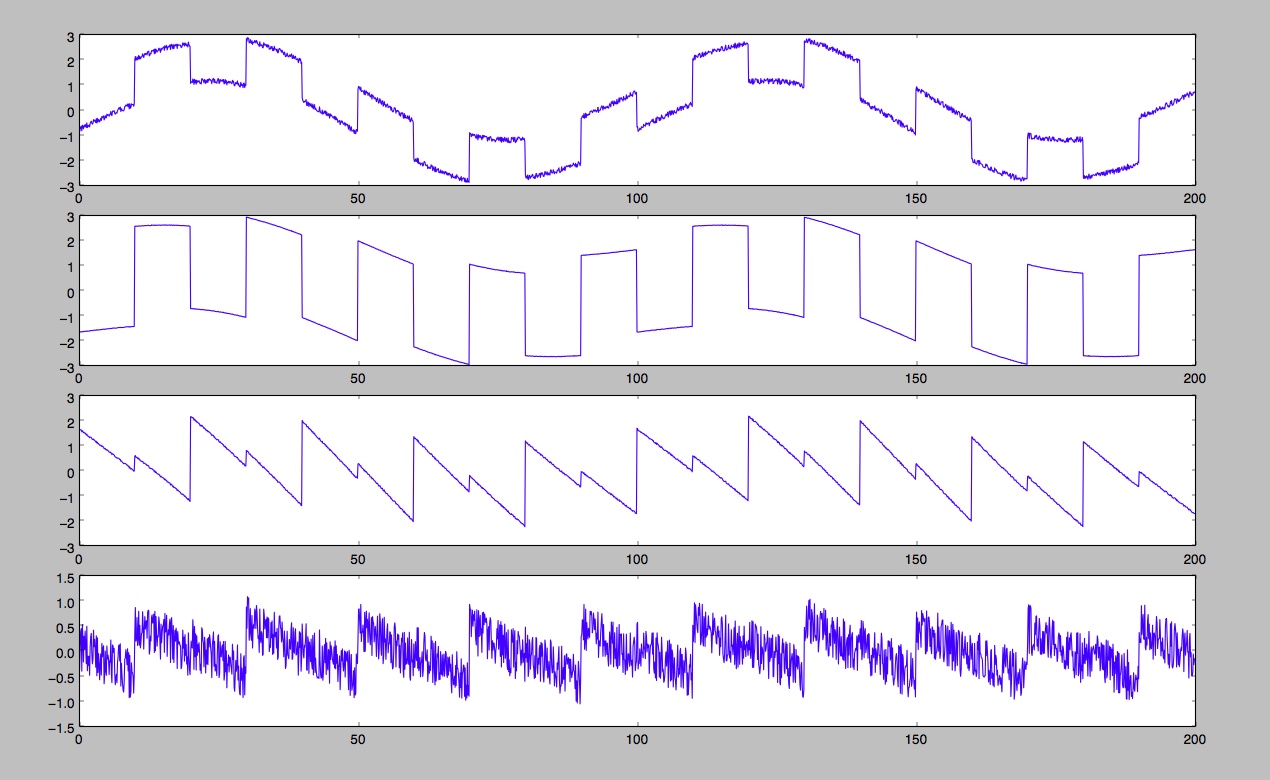
混合信号如下图:
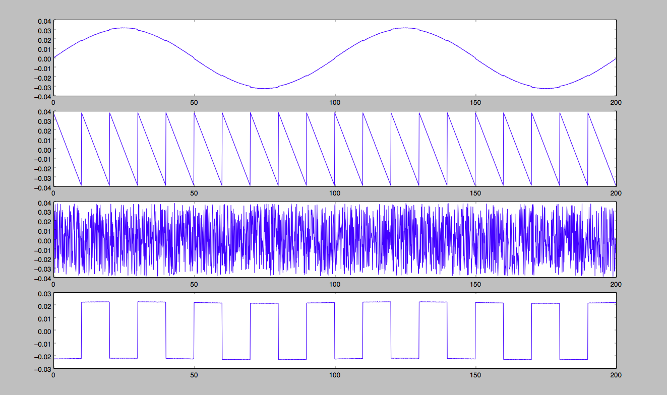
使用自己写的fastICA
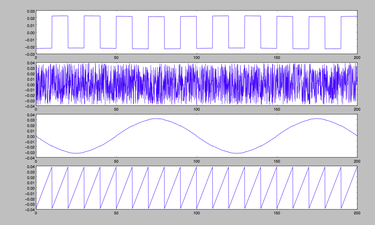
使用sklearn包里的fastica
参考
ICA(独立成分分析)在信号盲源分离中的应用
史上最直白的ICA教程
史上最直白的ICA教程pdf
Independent Component Analysis:
Algorithms and Applications
白化
Indepdent Componet analysis